How to Utilize Stars in Google Sheets to Enhance Scoring

Type @rating to include a wise chip in Google Sheets online for a viewer-friendly method to show zero-to-five star ratings.

Google Sheets lets you get in star rankings in cells with a wise chip. Given that many individuals discover stars much easier to separate at a glimpse than a list of numbers, this function might work any place you wish to rate items, functions, media, apps, locations or services. The function uses the exact same sort of 5-star format utilized in Android and Apple app shops and at Amazon, Uber and Yelp.

You might format cells for star rankings in Google Sheets online. As soon as formatted, you might pick and get in a ranking either in Google Sheets online or in the Google Sheets mobile apps on Apple or Android gadgets.

Dive to:

How to format a cell for stars in Google Sheets

Dealing with stars in a Google Sheet is a two-part procedure. Initially, you set up a cell to reveal stars, and after that you or your partners can get in a star ranking. To format a cell for rankings:

Open a Google Sheet in a web internet browser.
Location your cursor in a Google Sheet cell.
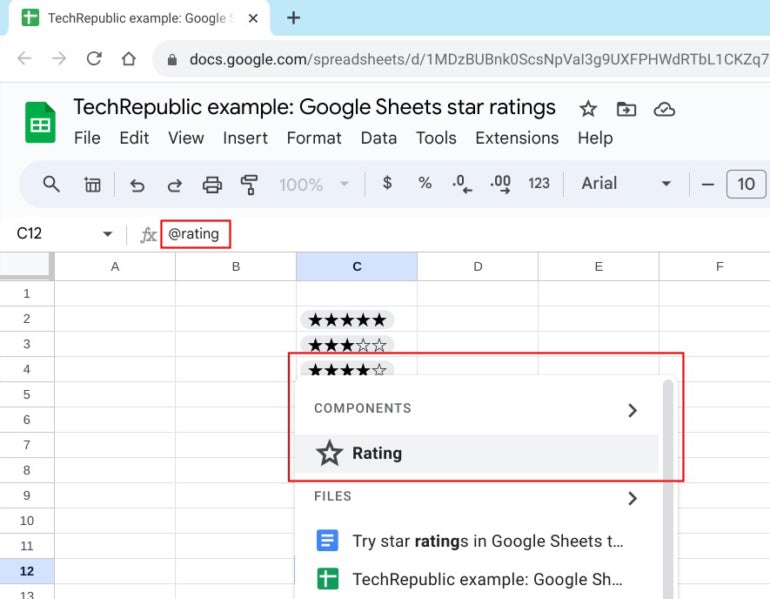
Type @rating and press return or get in to pick the star ranking element from the wise chip menu ( Figure A). The freshly formatted cell defaults to a mathematical worth of no and shows no stars.

Figure A

In Google Sheets on the web, use the @rating smart chip to format a cell for star ratings. — Figure A. In Google Sheets online, utilize the @rating wise chip to format a cell for star rankings. Image: Andy Wolber/TechRepublic

How to get in a star ranking in Google Sheets

As soon as a cell has actually been formatted to show a star ranking, you might get in the ranking either online or in Google Sheets on a mobile phone.

To get in stars while in a web internet browser, such as Google Chrome:

Click or tap on the cell formatted for stars.
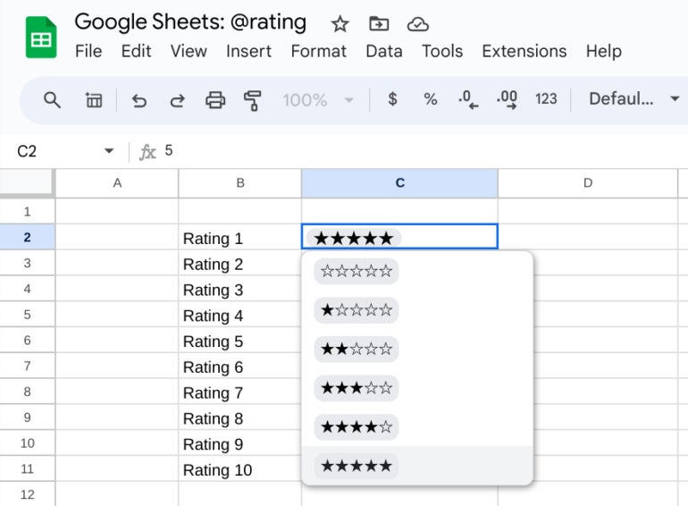
From the 6 menu choices that show, choose anywhere from 0 to 5 stars with a click or tap ( Figure B).

Figure B

In Google Sheets on the web, select an @rating cell, then choose a star rating option. — Figure B. In Google Sheets online, pick an @rating cell, then pick a star ranking choice. Image: Andy Wolber/TechRepublic

To get in stars in the Google Sheets mobile app on Android, iPhone or iPad:

Double tap on a cell formatted for stars.
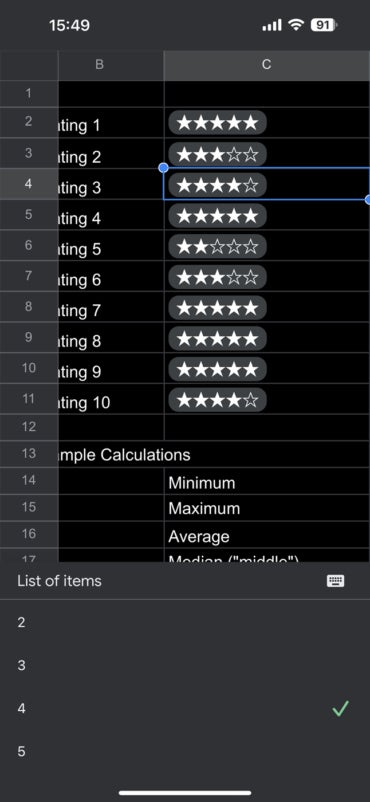
Select the variety of stars (i.e., 0 to 5) you wish to get in from the list that shows. You might require to scroll down the list a bit to tap on the greater numbers (i.e., 4 and 5) ( Figure C).

Figure C

In the Google Sheets mobile app, tap an @rating cell, then scroll and tap to select the number of desired stars. — Figure C. In the Google Sheets mobile app, tap an @rating cell, then scroll and tap to pick the variety of preferred stars. Image: Andy Wolber/TechRepublic

How to utilize a couple of solutions to examine star rankings

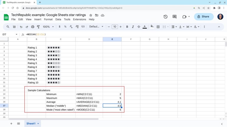
Rankings in Google Sheets are shown as the numbers no to 5, which indicates you might acquire worths from each star ranking cell. The following solutions can assist you examine a series of star rankings in Google Sheets ( Figure D).

Figure D

Since each rating corresponds to a number between 0 and 5, you may perform calculations with ratings such as MIN, MAX, AVERAGE, MEDIAN or MODE. — Figure D. Given that each ranking represents a number in between 0 and 5, you might carry out computations with rankings such as minutes, MAX, AVERAGE, MEAN or MODE. Image: Andy Wolber/TechRepublic

What are the most affordable and greatest rankings?

The Minutes and Max solutions return the most affordable and greatest numbers from a set, respectively. For instance:

= Minutes( C2: C11)

= Max( C2: C11)

The distinction in between the Minutes and Max shows the complete series of individuals’s rankings. For instance, a Minutes of 3 and a Max of 4 shows contract on a mid-range rating from responders, compared to a Minutes of 1 and a Max of 5, which indicates a larger series of rankings.

What is the typical ranking?

The average of a set of stars will be someplace in between 0 and 5, and can show the total agreement throughout all rankings. When comparing 2 rankings, the greater typical normally shows in general greater rankings. To determine the average, the system includes all rankings, then divides the overall by the variety of rankings gotten. For instance:

= Typical( C2: C11)

What is the middle ranking?

The mean is the worth that separates an embeded in half, with half of the rankings above the mean and half of the rankings listed below it. In contrast to the average, which can be impacted by a couple of very high or low rankings, you may think about the mean as dependably showing the middle of a set. To acquire the mean, utilize a formula such as:

= Average( C1: C11)

What ranking was most supplied?

Mode returns the ranking most often discovered in a set. For instance, in a set of 10 rankings, if 4 of those are 2 stars, 3 are 4 stars, and 3 are 5 star, the mode would be 2 stars. For instance:

= Mode( C2: C11)

Unlike the above solutions, which will constantly return an outcome, Mode may not. For instance, in a set of 10 rankings, if 2 individuals each ranked products one, 2, 3, 4 and 5 star, there would be no mode. Given that each of the possible rankings would have gotten 2 outcomes, there would be no single ranking that got one of the most. Likewise, if star rankings are divided in between 2 numbers (e.g., 5 individuals ranked a product as 4 stars, and 5 individuals ranked it as 5 star), once again, there would be no mode.

Reference or message me on Mastodon ( @awolber) to let me understand how you utilize star rankings and associated computations in Google Sheets.